Bragg-edge simulator
Introduction
This tool will simulate the Bragg edge spectrum of a given set of structures you can either import (.cif or config file) or manually define.
A full explanation can be found in our paper Applying neutron transmission physics and 3D statistical full-field model to understand 2D Bragg-edge imaging.
Tutorial
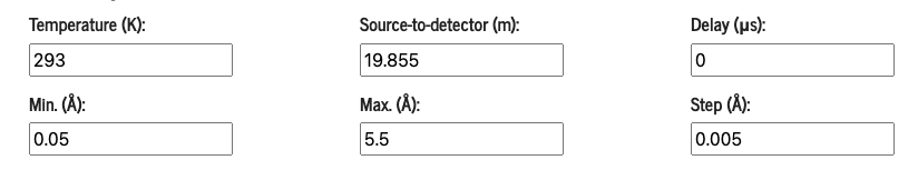
Global parameters
This is where you defined the x-axis of the data to plot as well as the experiment settings (distance source-to-detector and delay) and Temperature.
Input elements
Up to 5 different structures can be defined. Each structure is defined in its own tab
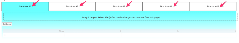
Structures can be defined 3 different ways
- manual input in the table
- import of a .cif file
- import of a config file saved in a previous session of that same tool.
Manual input in the table
If you want to manually enter the structure of your elements,
- select any of the empty structure tab,
- add a row (if there isn’t any empty row already) by clicking the add row button
- enter the atom name, h, k, and l values
Import structure via a .cif file
Simply drag & drop the ,cif file into the import widget.
Import a config file
Each config can be saved by clicking the Export structure button. This file can be re-imported by dragging & dropping it into the same import widget. In addition to filling the texture table, the config file will also set up the texture and grain size settings.
Texture
This option can be turned off. If checked, define as many hkl inputs as you want. For each, define at least one of the r and beta parameters.
Grain size (m)
This option can also be turned off. If checked, define the average size of the grains, in units of meters.
Structure parameters
This is where the a, b, and c distances are defined, as well as each alpha, beta, and gamma angle.
Export structure
Click export structure to create a JSON file format that you will be able to re-load into this application. This file will have all the parameters you defined for the given structure. 
Display profiles
Once all the structures have been defined, click the Submit button to display the profiles (be patient as it may take a few seconds to run the calculation and display the plots).
Bragg profiles
Feel free to play with the various axis (x and y options), scale options, and various plots (total, absorption only, coherent elastic scattering, coherent inelastic scattering, incoherent elastic, and, incoherent inelastic scattering).
Display data
Click Display plotted data to numerically see the data plotted.
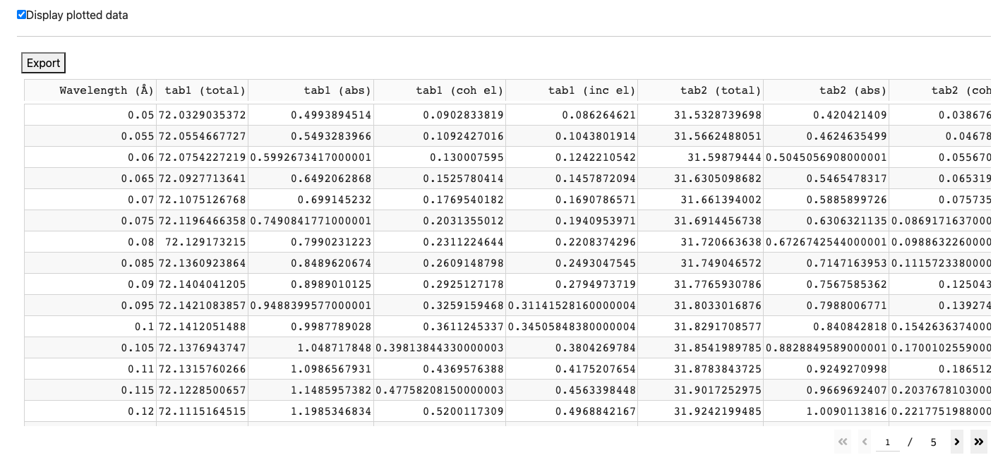
Click Export above the table to export this table into an JSON file.
Export all data as JSON
If you want to export all the structures and parameters used, click Export all data as JSON. This format can be easily used via Python and even display using a simple browser.
