Water intake Profile Calculator
Description
This notebook will calculate the water intake profile vs the time of a sample.
Here are the steps (bold for user input/manipulation)
- select the normalized images
- images sorted by time (by default)
- User Interface pops up!
- region of interest selected
- (optional) change the sorting algorithm
- by name
- by date
- (optional) select a folder containing the original .dsc files (which contain the right time stamp)
- profile of counts vs vertical-pixel calculated (select integrated algorithm: mean/median/sum)
- water intake profile vs file index or vs time
- export profiles
Tutorial
Select your IPTS
Need help using the IPTS selector?
Select images to process
Using the file selection tool, select the images your want to process. Once you click the Select button, the time stamp and the images will be automatically loaded. Wait for the progress bar to be done.
UI tutorial
Resizing widgets
It’s possible to resize or move any of the plots.
Sorting algorithms
By default, all the images are sorted using their time stamps. But in some cases (old IPTS), the time stamp may be wrong. So It’s possible to:
- either sort them using their name and let you define the time interval between the runs
- define a folder that contains the .dsc files created by the MCP. Those files contain in all cases, the correct time stamp.
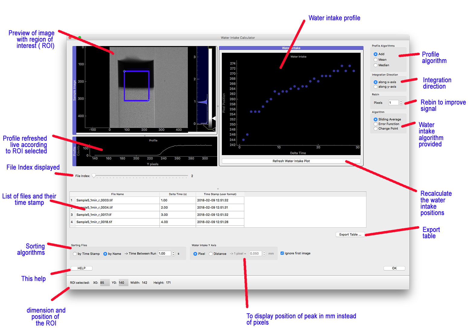
Profile algorithm
You can select the profile algorithm to use (to integrate over the x-axis of the region selected) using the profile algorithms available
- add
- mean
- median
The profile is calculated using the following method:
- retrieve the region you defined in the top left image
- using the profile algorithm you selected, will integrate over the x-axis of the ROI
- display the profile vs the y-pixels.
Using pixel or size reference
By default, the water intake profile displays the position of the “wave” as a pixel number vs the time. But it’s also possible to display this one using a real dimension (mm). To do so, just click the water intake y_axis -> distance check box and define the dimension of the pixel.
![]()
Integration direction
In the new version of the application, it is now possible to specify the direction of integration of the profiles. Select either y_axis or x_axis to change this direction.
Water intake algorithms
It’s possible to choose between 2 different algorithms to calculate the “wave” front position.
Sliding Average
This method is fully demonstrated in this PDF document
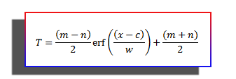
Error Function Fitting
The signal is fitted using a modified version of the error function as shown here
Change point
You can now select a 3rd algorithm based on the following python library (changepy)
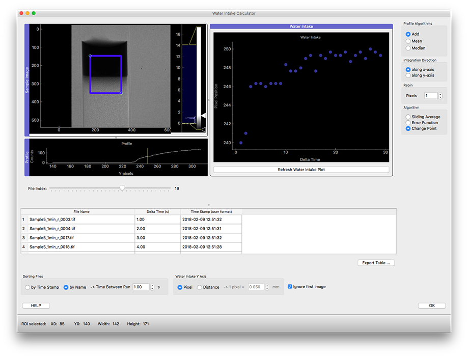
Rebin
For very poor statistics data, you can rebin the data by 2, 3, or more pixels. This will decrease the resolution of the water intake peak position but will improve its calculation by the various algorithms (sliding average, error function, …)
Live demo
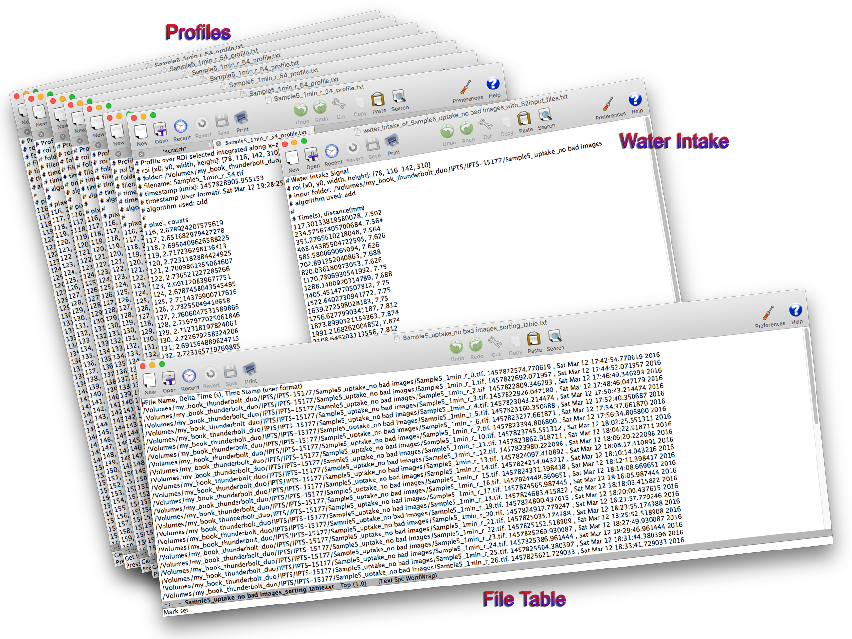
Export results
You can export the following data
- profile (Export > Profiles …)
- water intake (Export > Water Intake …)
- Table (Export Table …, on the right of the table)
For Advanced users, keep reading !
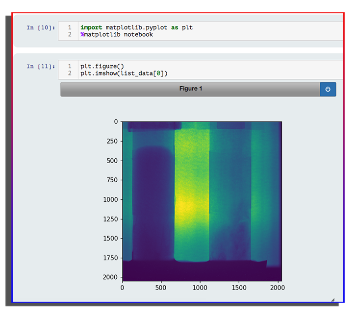
If you want to work on your data within the notebook
If you want to play yourself with the data loaded, you can easily access all the data and metadata loaded.
list_of_data = o_gui.dict_data['list_data']
list_of_files = o_gui.dict_data['list_images']
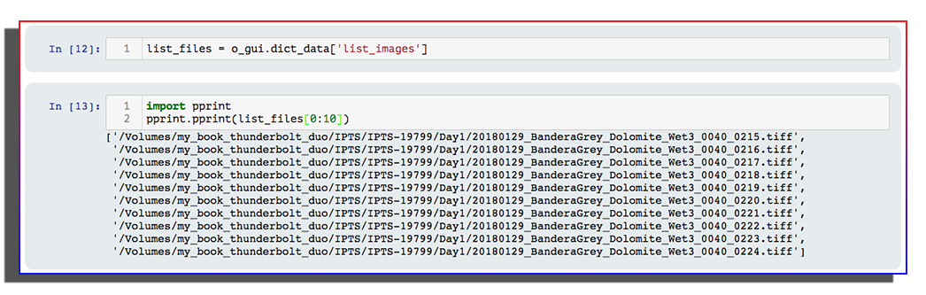
    list_of_time_stamp = o_gui.dict_data['list_time_stamp']
list_of_time_stamp_user_format = o_gui.dict_data['list_time_stamp_user_format']
