Wave front dynamics
Description
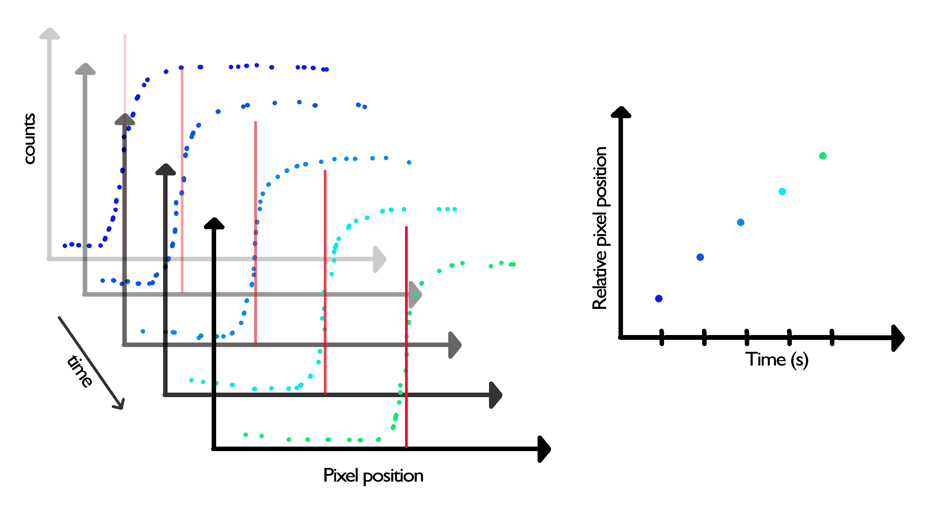
The main goal of this notebook is to follow the evolution of a wavefront over time.
The ASCII input data files supported by this notebook are produced by:
- the radial profile notebook.
- the linear profile notebook.
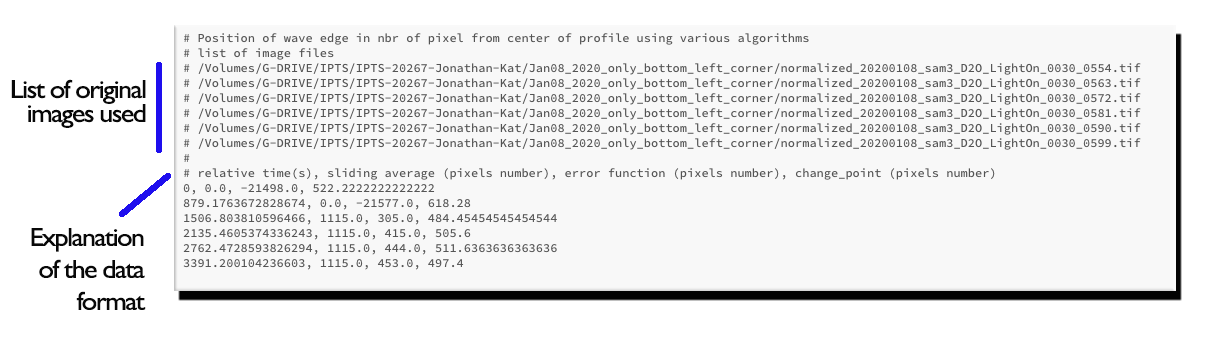
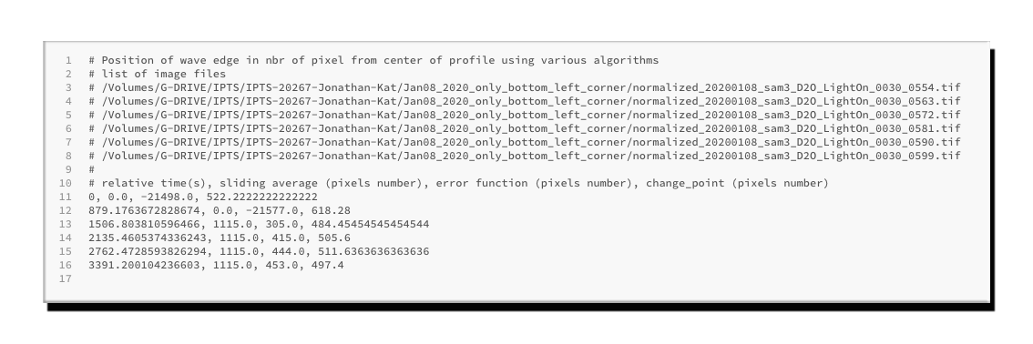
This notebook will output an ASCII file of the edge position according to the selected algorithms.
Tutorial
Select your IPTS
Need help using the IPTS selector?
Select profiles files to process
Using the file selection tool, select the profile files you created.
If you produced the input file using the radial profile notebook, feel free to select all the ASCII files (each corresponding to the radial profile of one single image). If the input file is coming from the linear profile notebook, only 1 ASCII file can be selected.
UI presentation
Running the next cell will bring the user interface (UI) to life.
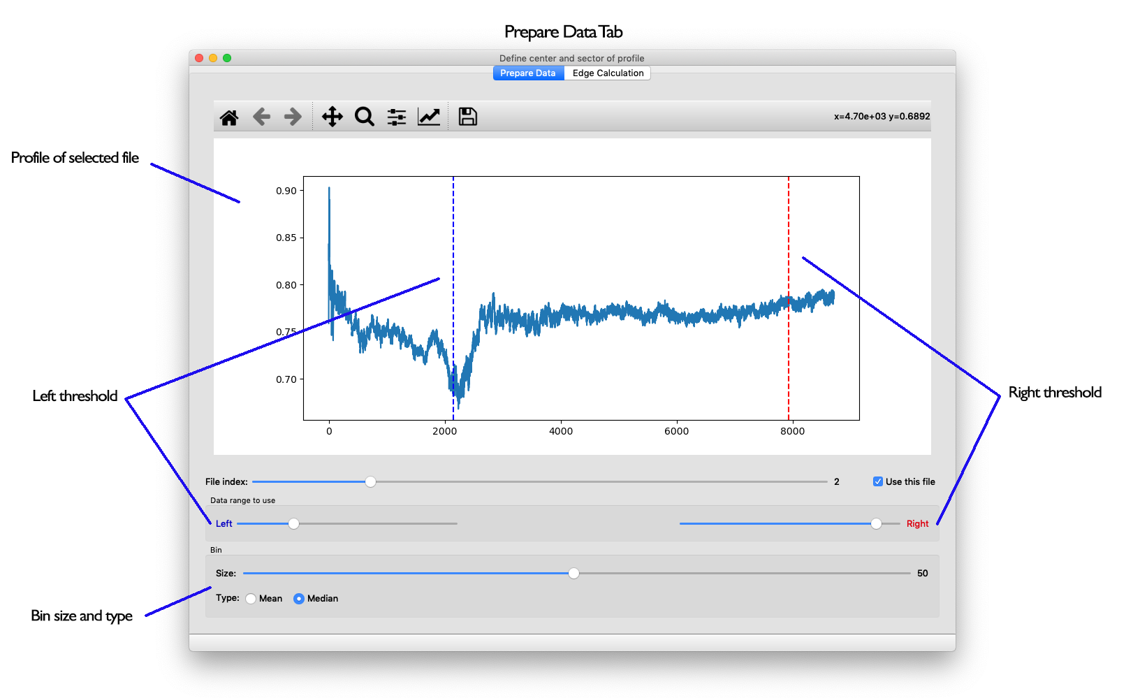
Prepare data tab
Step1
Make sure you want to perform the calculation on all the files loaded. If you want to exclude any of the files, select the file using the file index slider and turn off the Use this file checkbox.
Step 2
To help the algorithm, select the range of data to use to detect the edge and try to exclude any signal you don’t care.
Step 3
To improve statistics and speed, play with the rebin parameters (size and type). We noticed that in nearly all cases, binning will speed up the algorithms and will help find the right edge.
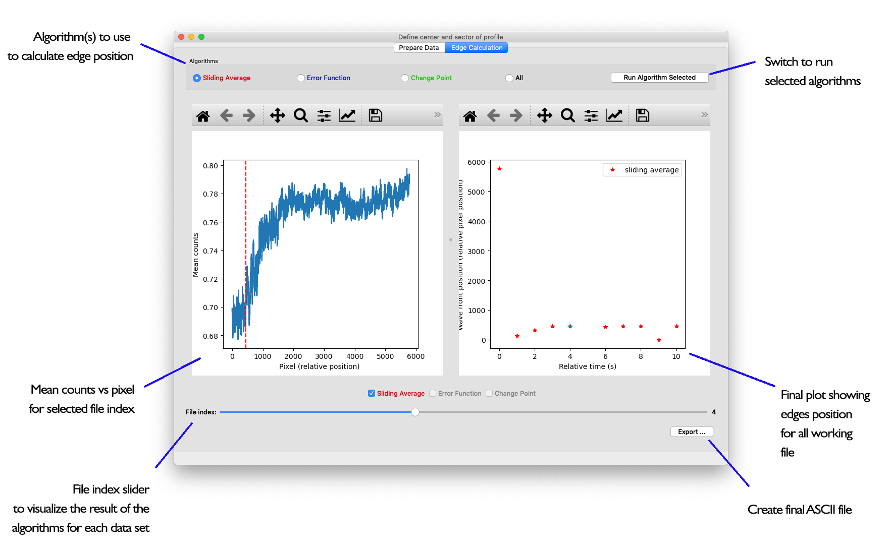
Edge calculation tab
Once you are done preparing the data, it’s time to detect the edge position. 3 algorithms are available and can be used at the same time to compare the results. Depending on the signal, such or such algorithm may work better than another one.
List of algorithms available
Sliding Average
Check the following document to learn about the algorithm behind it PDF document
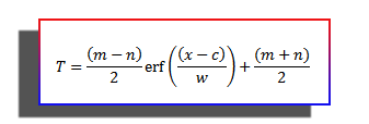
Error function
The signal is fitted using a modified version of the error function as shown here
Change point
This algorithm uses the following python library (changepy)
Run algorithms
Select the algorithms you want to use, or click *ALL to use all of them, then click Run Algorithm Selected
Export data
Click the Export … button to create the final ASCII file. Select the output folder and click OK.