Timepix3 – Histogram HDF5 MCP Detector
Description
The main goal of this notebook is to calibrate the instrument (detector-offset, distance source-detector, time-shift) by fitting a Bragg edge and aligning it with a well know Ni or Ta Bragg edge peaks.
Tutorial
Select your IPTS
Need help using the IPTS selector?
Prepare the user interface engine
Simply run this cell to prepare the notebook for the ROI selection (later in the notebook)
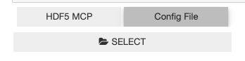
Select Input File
At this point, you have the option to either select a HDF5 MCP histogram file (created by the notebook From event to histo hdf5) or a config file (created during the last step of this same notebook).
Select the type of file you want to load and then click the SELECT button to start the process.
Select HDF5 MCP histogram file
Using the file selection tool, select the histogram HDF5 file created by the from_event_to_histo_hdf5 notebook.
The file will then be automatically loaded.
Select config file
If you already ran this notebook all the way until the end, you then had the option to save the session. This is the file you can load here. This will automatically re-use the parameters (for example, detector-offset, time-shift, fitting parameters, etc.) defined during that session.
Using the file selection tool to select that file (extension being .cfg).
Integrate signal
To get a preview of the stack integrated over the time_of_light axis, run the cell.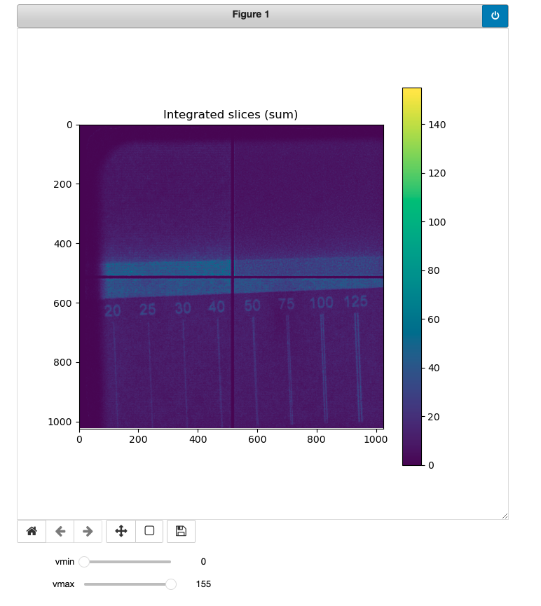
Select 1 or more region(s) of interest (ROI)
This or those regions will be combined, for each image, and averaged in order to give 1 value per image. This will produce the profile we will work on in the rest of the notebook.
Running the cell will pop up a window (which may be hidden behind the browser) where you must select at least one
Display profiles of ROIs
The integrated image with the ROIs selected will be displayed at the top of that cell. Using color matching, the profiles of the respective ROI are shown in the bottom part of the cell.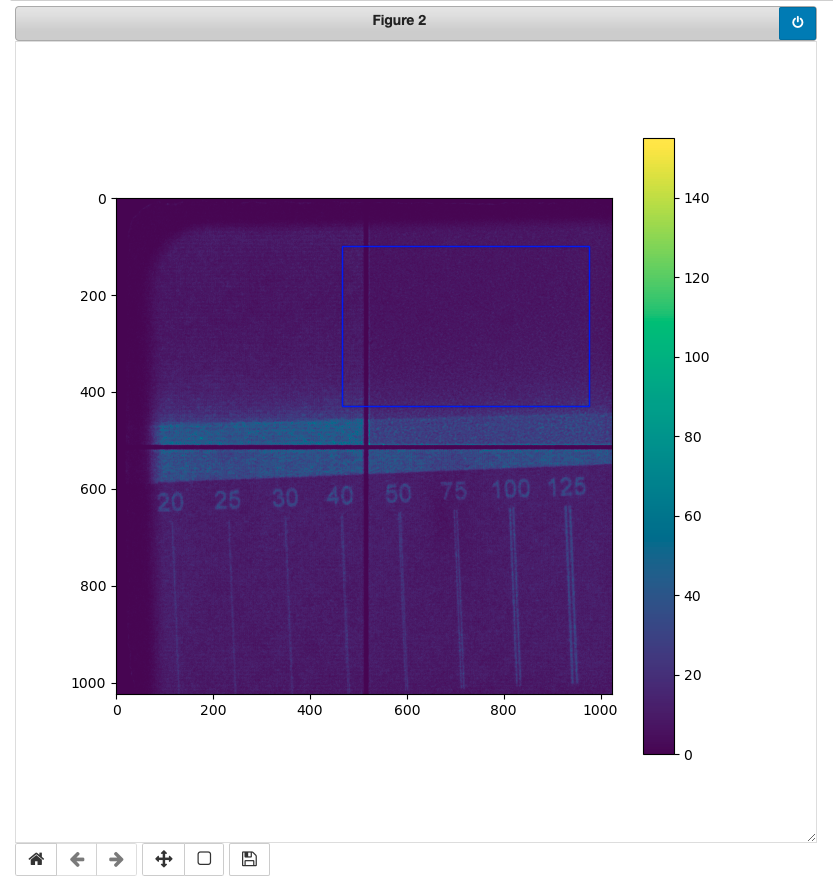
This is where you can play with various parameters, such as x-axis units, distance source-detector, detector offset, time-offset. You can also overlap the profile with the first 6 Bragg edges of Ta or Ni.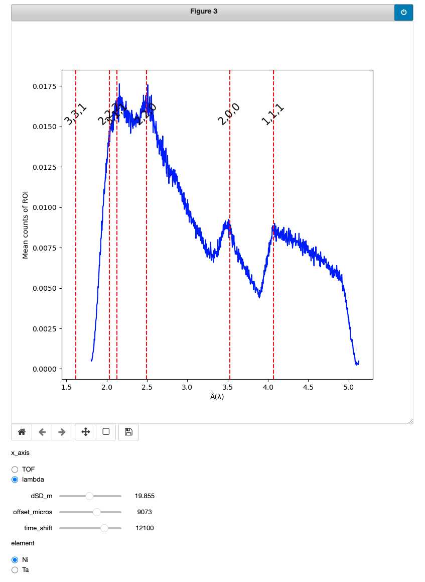
Fig Bragg peak
The following steps will allow you to fit any, one at a time, of the Bragg edges. 2 steps will be required:
- Select the full range around the Bragg edge peak as well as the edge of the peak
- Define the initial fitting parameters
1.Select peak to fit
Using the sliders, place the left and right range (green lines) around the full peak (as shown in the following screenshot). Then using the left and right edge (red lines) sliders, define the peak itself. 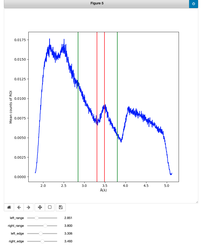
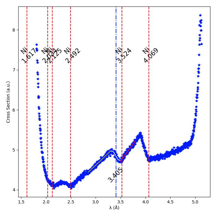
2. fit peak
Play with the input parameters (if needed) and click FIT to fit the peak you selected. 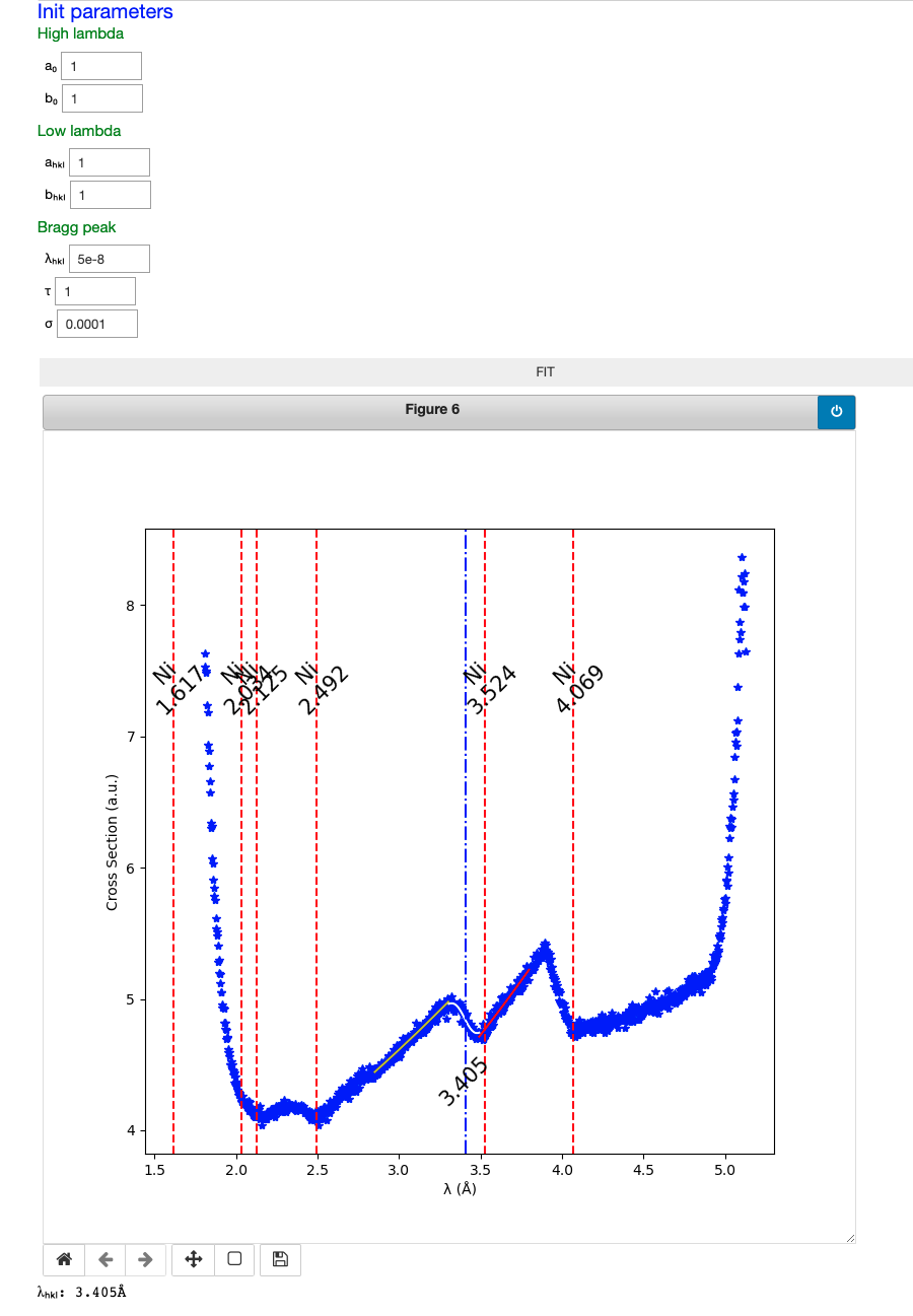
The fitted lambda will be highlighted as a vertical blue line, while the Bragg peaks of the element selected will be displayed as well.
The value of this calculated lambda is also displayed at the bottom of the plot.
99% of the time you will only need to try different input values of λhkl (5e-9, 5e-7, 5e-6) and σ (.01, 0.0001, 0.001) if the fitting does not work.
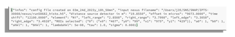
Saving session
This is where you can save all the parameters, regions of interest, ranges, etc., defined during the current session. This will allow you to reload and replay the current session the next time you restart the notebook.
Using the folder selection tool, select where you want to create this config file.
The config file name will be based on the input HDF5 file name with the addition of a time stamp.
input hdf5 file name: run58682_histo.h5
config file name: config_run58682_histo_03m_24d_2023y_10h_38mn.cfg