Cylindrical Geometry Correction with Embedded Widgets
Description
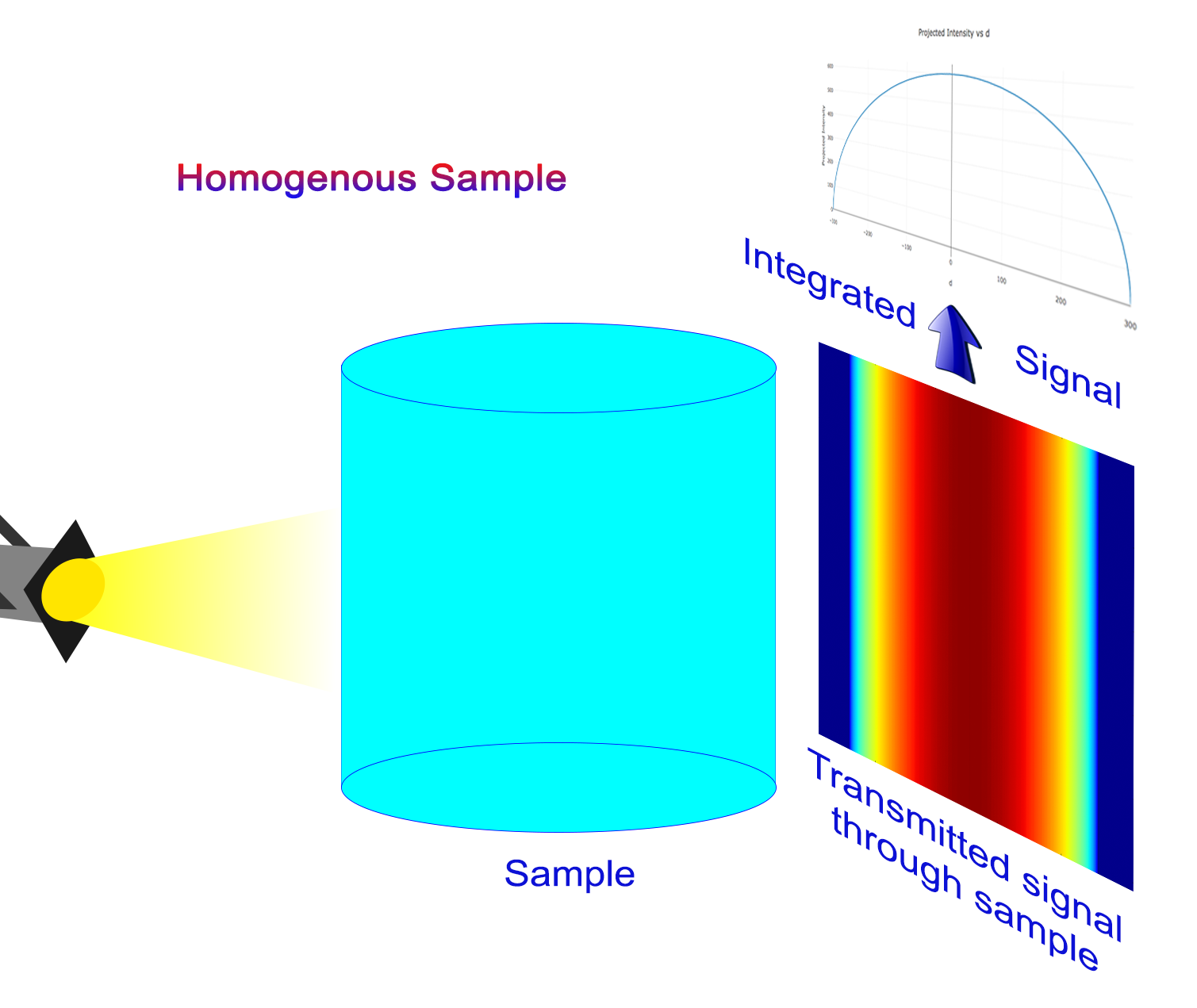
If a homogenous sample is cylindrical, the data will show an inhomogeneous transmission signal due to the fact that the neutron beam has to go through more material at the center compared to the side. This notebook corrects this inhomogeneity.
This notebook is using a library developed by the neutron imaging team and located on GitHub.
Tutorial
Workflow of the notebook
The workflow of the notebook is explained in this first cell showing the optional cells, and the user steps where some interaction is requested from the user.
- User: select the images to work with.
- Notebook: load images
- OPTIONAL: User load config file
- User: rotate the images to make sure the sample to work with is perfectly vertical
- User: select region to work with by cropping the raw data
- OPTIONAL: User export the cropped images
- User: select part of the image that does not contain the sample
- User: select part of the image that does contain the sample
- Notebook: remove background from the sample part
- Notebook: display profiles
- Notebook: apply geometry correction to all profiles
- User: select where to output the images corrected, profiles ASCII files, metadata file, and config file.
Select your IPTS
Need help using the IPTS selector?
Select Images
Using the file selection tool, select the images you want to work with.
Use Config file (OPTIONAL)
In the case you already ran the notebook with the same set of data, you can reload a config file that will automatically default all the ROIs to the value found in the config file.
If you don’t want to load any config file, just skip that cell.
Visualize Raw Data
This is where the data are displayed to make sure you are working with the right data set. Feel free to use the slider at the bottom to browse through the data loaded.
Rotate the sample to make sure it’s perfectly vertical
To make sure the algorithm works, the same MUST BE perfectly VERTICAL. To find the perfect vertical of your sample, a set of tools are provided, such as the vertical guide and the two horizontal profiles.
The vertical guide can be moved around and will give you a visual indication of the verticality of the sample.
The 2 horizontal profiles are here to display the horizontal profiles (green and blue dash lines). A perfect superposition of the two profiles indicates that the vertical is perfectly vertical (as demonstrated in the following animation).
On the right, the region around the vertical guide is displayed in order to help figure out the perfect rotation parameter to use to get a perfectly vertical sample.
Crop sample to region of interest
This is where you need to select only the sample by keeping in mind the two following conditions:
- make sure the container is included in the selection. Because we are working with normalized data, the edge should have a value of 1
- make sure a part of the container without the sample in the field of view is also selected. This will be used in the normalization to remove the container from the signal.
LIVE DEMO
Export cropped images (OPTIONAL)
You have the option to export the cropped images as TIFF files here. Simply use the folder selection tool to define the output location where the cropped images will be exported.
Select background
In order to perform the geometry correction, the program needs to know which part of your cropped images is the background and which part is the sample.
In this cell, you select the background.
Select sample
Following the same process, select the part of the sample that only contains the sample. This is also the part that will be corrected.
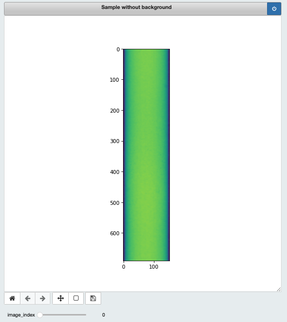
Removing tube background from sample
This cell will take care of removing the signal due to the sample environment to the rest of the data. This will leave us with only the signal from the data itself.
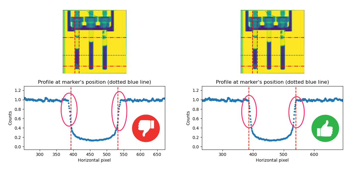
Profiles to work with
Just to make sure we selected the right region of interest (ROIs), this cell displays the various profiles along the height.
Applying geometry correction
The correction to the sample data is applied using the algorithm implemented in our cylindrical geometry correction library
Export
This is where you will export:
- The corrected cropped images (tiff format)
- The full horizontal profiles of each image (ASCII format)
- The configuration file (JSON file format). This is the file you can reload at the top of the notebook to automatically use the same region of interest you have been using in this session.
Use the folder selection tool to define the location where all those files will be exported.
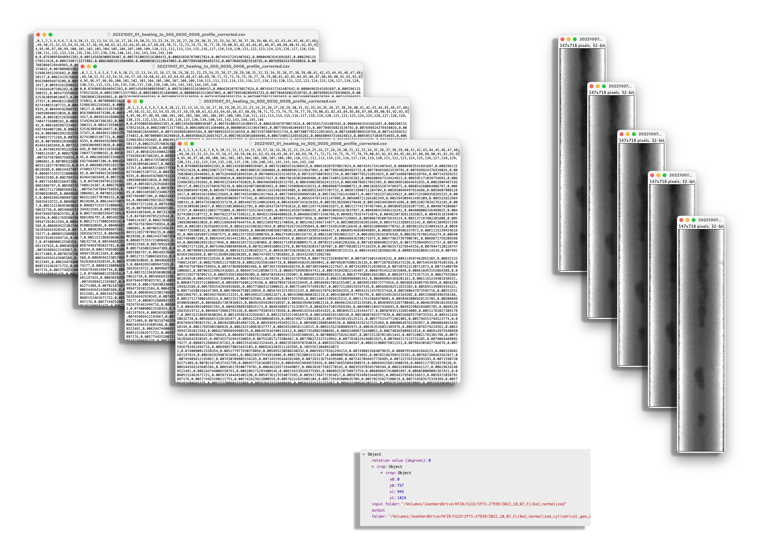
The value produced in the ASCII file corresponds to the attenuation per pixel.
