Panoramic stitching for TOF
Description
This notebook stitches images acquired in TOF mode.
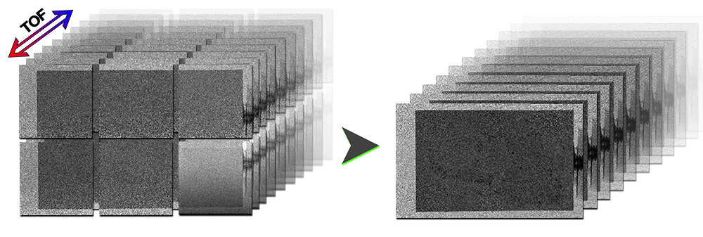
The notebook takes a set of folders as input. Each folder corresponds to a different coverage of the sample and contains all the TOF images acquired using the MCP detector. You will need to manually position either the integrated signal over all the TOF, or the best contrast image (calculated using the Dual-energy algorithm described in the notebook dual energy). Then the program will stitch every single TOF image using those same parameters. In the end, you will have a folder of the stitch images with as many images as any of the input folders.
Tutorial
Select your IPTS
Need help using the IPTS selector?
Select folders to process
Using the folder selection tool, select all the folders you want to use. Each folder must contain the TIFF images of single panoramic stitching (all the images of that folder will be stitched together).
User interface
Step 1 – Select the stack of images to work with
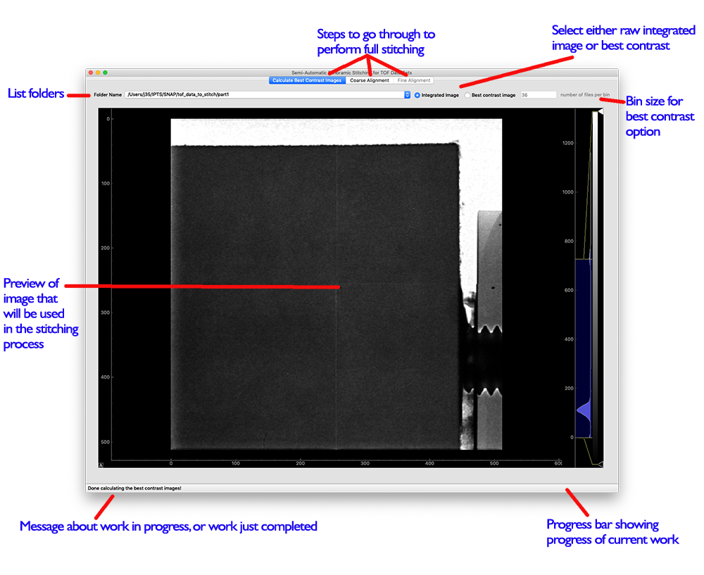
The first tab Calculate best contrast images allows you to determine the images with the best contrast. 2 options are offered:
- Integrated image
- Best contrast image
The Integrated images are for each folder selected as the sum of all the images. The best contrast image uses the algorithm defined in the dual energy notebook). Feel free to play with the binning size to improve the contrast. Once you are happy with the image mode you selected, just move on to the next tab Coarse alignment.
Step 2 – coarse alignment
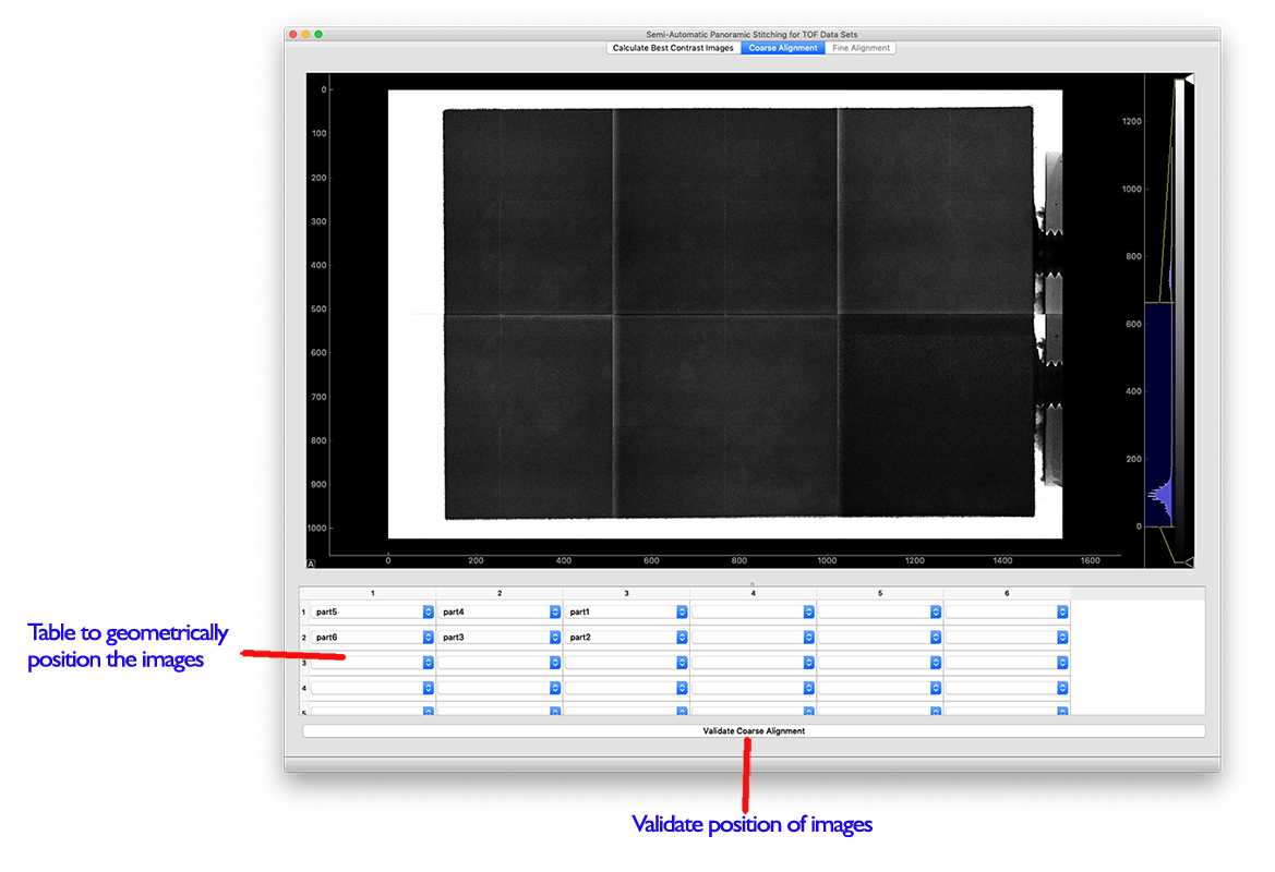
Because the images produced in TOF mode do not have the position of the motor as metadata, it’s up to you to roughly determine their position using the table. Just select all the images, and only one time, and position them relative to each other. Once you are happy with your selection, click the Validate Coarse Alignment button to record those positions. You can now move on to the next and final step.
Step 3 – Fine alignment

The top left corner image, first image/file from the list, is fixed. This is the reason why selecting the first raw in the table will display a blue border around the image.

Any other row selected will display a red border around the image selected. You have three options to move those images.
- using the mouse
- using the manual offset button to jump by 1 or 5 pixels at a time
- entering offset values directly in the table
Using the Mouse
To activate the mouse mode, click the From -> To pointer switch at the top of the UI. This will brings a couple of target labels FROM and TO within the panoramic view. Simply move the FROM target within the image selected region, inside the red box, to a feature you recognized in the previous image stitching. Move the TO target to that same feature and then click Move image of active row FROM -> TO to reposition that image.
the Move image of active row FROM ->TO button will be enabled only when the FROM target is within the image selected (surrounded by a red border).
The UI provides a horizontal and vertical profiler tool to help in the alignment of 2 images.
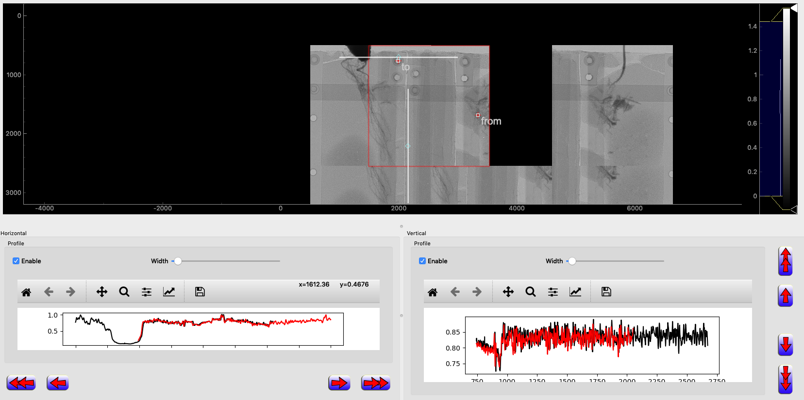
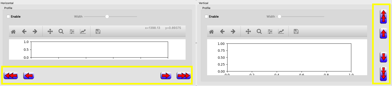
Feel free to move around the horizontal and vertical profilers, and resize them in length or width as illustrated here.
The BLACK plot shows the profile from the reference image, the RED plot shows the profile of the working image.
Using manual offset buttons
Using those buttons, you can move the working image by 1 or 5pixels at a time horizontally or vertically.
Using table
You can also directly enter the xoffset or yoffset of any image, except the first one, within the table. Double click the field you want to edit to change the x or y offset.
Export panoramic images
You can now repeat the alignment on all the TOF slices by clicking the Export Panoramic Images button. You will need to select the output folder where you want to create the final folder which will be named after the parent input folder’s name.
For the region of overlap between two images, the notebook simply takes the average of the two images.
